Introduction
A control system consists of interconnected components which is designed to achieve a desired purpose. To understand the purpose of a control system, it is useful to examine examples of control systems through the course of history. These early systems incorporated many of the same ideas of feedback that are in use today.
Modern control engineering practice includes the use of control design strategies for improving manufacturing processes, the efficiency of energy use, advanced automobile control, including rapid transit, among others.
Theory
A control system is a device, or set of devices, that manages, commands, directs or regulates the behaviour of other device(s) or system(s). Industrial control systems are used in industrial production for controlling an equipment or a machine.
Control systems are components that are added to other components, to increase functionality, or to meet a set of design criteria.
Example :
We have a particular electric motor that is supposed to run at a rate of 40 RPM. To achieve this speed, we must supply 10 Volts to the motor terminals. However, with 10 volts supplied to the motor at rest, it takes 30 seconds for our motor to get up to speed. This is valuable time lost.
This simple example, however can be complex to both users and designers of the motor system. It may seem obvious that the motor should start at a higher voltage, so that it accelerates faster. Then we can reduce the supply back down to 10 volts once it reaches ideal speed.
This is clearly a simplistic example, but it illustrates an important point: we can add special "Controller units" to pre-existing systems, to improve performance and meet new system specifications.
There are two common classes of control systems, open loop control systems and closed loop control systems. In open loop control systems output is generated based on inputs.
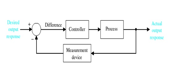
An open-loop control system utilizes a controller or control actuator to obtain the desired response . An example of an open-loop control system is an electric toaster.
In closed loop control systems current output is taken into consideration and corrections are made based on feedback. A closed loop control system is also called a feedback control system. The human body is a classic example of feedback control system. The term "control system" may be applied to the essentially manual controls that allow an operator, for example, to close and open a hydraulic press, perhaps including logic so that it cannot be moved unless safety guards are in place. Some terms related to control system are:
Variables- are used to control the quantities or conditions that are measured and controlled.
Process - is a natural, progressively continuing operation marked by a series of gradual changes that succeed one another in a relatively fixed way and lead toward certain result or end.
System– An interconnection of elements and devices for a desired purpose.
Control System – An interconnection of components forming a system configuration that will provide a desired response.

A plant in control theory is the combination of process and actuator. A plant is often referred to with a transfer function (not uncommonly in the s-domain) which indicates the relation between an input signal and the output signal of a system without feedback, commonly determined by physical properties of the system. An example would be an actuator with its transfer of the input of the actuator to its physical displacement. In a system with feedback, the plant still has the same transfer function, but a control unit and a feedback loop (with their respective transfer functions) are added to the system.

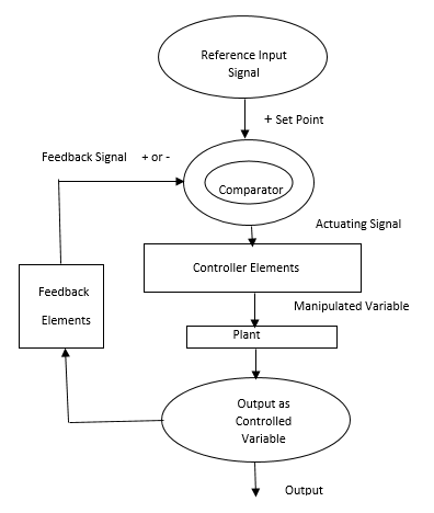
Fig:Flowchart of Control System
Control system in which the output has an effect on the input quantity in such a manner that the input quantity will adjust itself based on the output generated is called closed loop control system.
Figure above shows the Flow chart of control system in which feedback is taken from output and fed in to input.
In any control system, output is affected due to change in environmental condition or any kind of disturbance. So one signal is taken from output and is fed back to the input. This signal is compared with reference input and then error signal is generated. This error signal is applied to controller and output is corrected. Such a system is called feedback system.
Practical Applications of Closed Loop Control System are:
1.
Automatic Electric Iron– Heating elements are controlled by output temperature of the iron.
2.
Servo Voltage Stabilizer– Voltage controller operates depending upon output voltage of the system.
3.
Water Level Controller– Input water is controlled by water level of the reservoir.
4.
Missile Launched & Auto Tracked by Radar– The direction of missile is controlled by comparing the target and position of the missile.
5.
An Air Conditioner – An air conditioner functions depending upon the temperature of the room.
6.
Cooling System in Car– It operates depending upon the temperature which it controls.
Manual
Scilab is a programming language associated with a rich collection of numerical algorithms covering many aspects of scientific computing problems.
Whatever your platform is (i.e. Windows, Linux or Mac), Scilab binaries can be downloaded directly from the Scilab homepage
or from the
Download area.
Scilab elementary mathematical operators:
+ addition
- subtraction
* multiplication
/ right division, i.e. x/y =xy-1
\ left division, i.e. x\y = x-1y
^ power, i.e. xy
** power (same as ^)
' transpose conjugate
num is the numerator.
den is the denominator.
Here we use syslin command, syslin defines a linear system as a list and checks consistency of data. dom='c' for a continuous time system, dom='d' for a discrete time system, n for a sampled system with sampling period n (in seconds), dom=[] if the time domain is undefined.
Numerical simulation is nowadays essential in system design process. Complex phenomena simulation (physical, mechanical, electronics, etc.) allows the study of their behaviour and results without having to conduct costly real experiments. Widely used in the world of industry, the future generation of engineers and scientists are trained since secondary school to the concepts of modelling and simulation.
Xcos is Scilab tool dedicated to the modelling and simulation of hybrid dynamic systems including both continuous and discrete models. It also allows simulating systems governed by explicit equations (causal simulation) and implicit equations (a causal simulation). Xcos includes a graphical editor which allows to easily represent models as block diagrams by connecting the blocks to each other. Each block represents a predefined basic function or a user--‐defined one.
Xcos opens by default with two windows:
• A palette browser which provides a set of predefined blocks.
• An editing window which is the working space to design diagrams.
To design a diagram, just select blocks in the palette browser and position them in the editing window (click, drag and drop). Blocks are then connected to each other using their different ports (input, output, event) in order to simulate the created model.
Procedure
- To construct this plant in Scilab workspace, start with a seed ‘s’ representing Laplace variable.
- s=poly(0,'s')
- Then we can build on s any polynomial or rational function.
P=2/(s*(s+0.5))
- At this point, our plant appears like a rational function , but is not yet a linear transfer function that Scilab could interpret. We need to do one more step by using syslin command.
P=syslin('c',P)
- Suppose we have a controller
- Construct it in Scilab
C=syslin('c',(s+1)/(s+10))
- To compute a loop transfer function
L= C*P
- With this plant and controller, we now want to simulate how the closed-loop system behave in time-domain. The most common to observe is a response to step command. So we have to create an Xcos simulation model. Type xcos at Scilab command prompt to open a blank untitled window. Then open the Palette browser from View menu, find and drag the following palettes to the blank Xcos model:
• STEP_FUNCTION and CLOCK_c from Sources Palettes
• CSCOPE from Sinks Palettes
• MUX from Signal Routing Palettes
• BIGSOM_f from Mathematical Operations Palettes
• CLR from Continuous time systems Palettes
• TEXT_f from Annotations Palettes (optional)
- Connect the diagram as shown in Fig. The black and red signal routes cannot be mixed. Here we have red line only to the scope representing simulation clock. It is a good practice to label the blocks and signals with TEXT_f so that your diagram is understandable to others, but not required for the simulation to work.
- The CLR block needs data in the form of numerator and denominator polynomials.
-->P.num
ans=
2
-->P.den
ans=
2
0.5s + s
So we simply put C.num, C.den and P.num, P.den into the controller and plant CLR blocks, respectively, as shown in Fig
-
Try adjusting the Y-axis range of scope to Ymin = 0, Ymax = 2. Set final integration time = 30 (and set the scope Refresh period to match). Run the simulation and see what happens then readjust them.
The resulting response is unstable.
Output :